NTA2: NumericalTextAnalysisOrHamletQuestion

Numerical Text Analysis 2
Guide to all Text Analysis posts
Prev: Preliminaries
How the first line of Hamlet's soliloquy at the beginning of Act 3 Scene 1 of the eponymous play becomes {question: 1}.

Consider a text, either a web document, an essay, a personal profile or a book, e.g. Alice in Wonderland. It is a sequence of words (woRds, wodrs, wd.s, 'words?' and 9) separated by whitespace. Before doing any numerical work, we have to standardize the text using the text operations we described in NumericalTextAnalysisPreliminaries.

Here is what we know or what we should follow:

Don't create more word tokens.

Lower, since it commutes with all other operators and can be applied to the whole text, should be first.

Stem needs to come after DePunctuation, and since it operates on words, after Parse. Stop[rank] should be used after all the rest of the cleaning-up, and since the rank is to be determined based on word frequencies, should be after Parse and Histogram. Histogram should come after Stem. Chop[n] is not needed. I don't know what to do about abbreviations and mis-spellings, so I'll ignore those for now.

Standardization

1. DePunctuate (All punctuation but '-' deleted, '-' replaced by single space.) These first two steps can act on either text or lists.
2. Lower. The first two together are cummings.
3. Parse (on whitespace)
4. Stem (Porter2 from stemming package in Python by Matt Chaput)
5. Histogram Can act on either text or word list.
6. Stop[rank] Look at the Zipf plots of the histogram for the whole corpus to determine the rank of the word token below which words are to be dropped.
7. DeRarify
   
   
   First let me show you the Zipf plots for the text as we sequentially process it. Recall from the post on To Zipf or not to Zipf that it is a plot of the log of the product of the frequency and rank for any token vs log(rank). We expect it to be linear, indicating a negative power law dependence of the frequency on the rank.
   
   
   All processing is done using Python code, which also creates data files and calls R for plotting. When I get my hands on real data, the R program can also fit the data to Zipf's law or Mandelbrot's law, which will help with identifying the deviations from expected linear behaviour and the ranks at which we establish the 'stop' and 'rare' cut-offs. (To see more details of the figures and tables, click on them.)
   

   

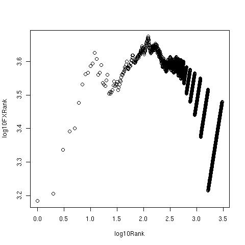
   Zipf Plot of Alice, original text

     From right to left, the different segments correspond to tokens which appear only once, then those that appear twice, thrice etc. The most frequent word 'the' sits at the bottom left corner. With a large corpus, we expect the curve to be smoothed out, especially in the middle.
   
   
   

   

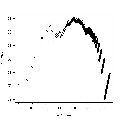
   Zipf Plot of Alice, text with punctuation removed

   
   

   

   Zipf Plot of Alice, lowercased text

   
   

   

   Zipf Plot of Alice, histogram of stemmed tokens

   
   

   

   Zipf Plot of Alice, histogram with 100 stop words removed

   
   
   
   
8. These 100 'stop' words are just the 100 most frequent words in the text itself. As I have explained in the Zipf post, the cut off should be based on the histogram of the entire corpus.
   
    Again, this is for illustration purposes only.
   

   

   Zipf Plot of Alice, histogram with 20 rare words removed

Now, let's take a look at the 20 top and 20 bottom ranked tokens in Alice, and see how this list changes with processing.



Top 20 Tokens



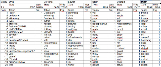Bottom 20 Tokens

 Summarizing,

The above steps suffice for spell-checked and edited works, the following steps need to be implemented for user provided text.
7.  Expand any recognizable abbr to its most likely form, so there is no remaining ambiguity. (I am not sure about this step, but presumably it involves looking up some standard dictionary.) From the remaining sequences of letters, identify the non-words and check if there are any likely words in the dictionary that could have been misspelled as the non-word. For example, consider the non-word 'mnager'. Let's say that 'manager' is likely to be misspelled as 'mnager' (dropped letter 'a') 5% of the time (where the probabilities over all result words – spellings and misspellings – of the source word 'manager' sum to 1), whereas 'manger' is likely to be misspelled as 'mnager' ('a' and 'n' transposed dyslexically) 10% of the time. These are not the probabilities to consider and thence assign 'mnager' to 'manger'. Since 'manager' is a much more frequently used word than is 'manger', 'mnager' is much more likely to be a misspelling of 'manager'. So we want to look at the probabilities that 'mnager' results as a misspelling of a source word ('manager' or 'manger'), where the sum over all source words equals 1, and then select the most likely source. Hence 'mnager' would be assigned to 'manager', unless one were to have additional information, e.g. that the text is biblical in nature.
8. Toss out 'fzdurq' and other non-words., so that all remaining sequences of letters are words.
   These last two complicated steps can be substituted by the step of simply removing the letter sequences which are least frequent in the corpus, which are either terms from highly specialized jargon, mis-spellings or abreviations.

So you see how “To be, or not to be, that is the question:” is rendered “question”. The corpus of the text remains; ready for some numerical, but not literary, analysis.

Next: Selecting Stop Tokens