Friday, March 30, 2012

NTA7:Dimensional Sparseness Or What Tokens To Use?

NTA7: Dimensional Sparseness Or What Tokens To Use?

Guide to all Numerical Text Analysis posts

 Word histogram and Zipf plot of corpus for identifying stop words

After
  • lowercasing,
  • depunctuating,
  • removing single atom words,
  • removing single occurrence tokens,
  • stemming and removing a few stop words (whether the 125 I have chosen or the ~ 450 in standard lists,
we are left with about 14000 tokens from a bit less than 100 documents.

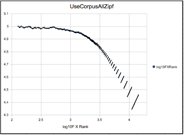
Here is the Zipf plot:


Before going on to the Cosine Similarity business, let's think about Word-vector space. Each token represents a dimension, the frequency of occurrence is the coordinate. Each document represents a point in this space. So what we have is a 14,000 dimensional space for a 100 points. That's ridiculous! But let's consider we have a million documents, that is still only 70 points per dimension!

Now of course this is going to vary from case to case, e.g. the categorization problem I worked on had 25,000 points in 50,000 dimensions. Hardly a situation where standard clustering algorithms – most of which are designed for denser graphs (at least dimensionally speaking) can be expected to apply. My solution to this is on SlideShare, and I'll blob on it at length later.

My point, as was my point for selecting stop words, is that some [statistical or numerical] and purpose-based criteria have to be used to decide which set of tokens to use. If you look at the Zipf plot above, in my view there are clearly three families of tokens:
  • the high ranking ones that approximate a Zipf line with a coefficient marginally less than 1

  • the mid ranking tokens at the knee of the plot which fall off the Zipf line

  • the low ranking tokens whose power law deviates very strongly from 1


My choices for the cutoffs are somewhat arbitrary, but unimportant for now. Summarizing,


What do these mean? Consider the extremely rare ones that occur only once in the corpus, and hence in only one document. So they are extremely powerful for distinguishing one document from another and a reasonably small set of these plus a few that occur a few times (There may be a few documents which contain no singly occurring tokens.) will be sufficient to label every document uniquely. However, precisely because of their rarity, we can't use them for finding any similarities between texts. So these low ranking tokens lead to a very fine-graining of the set of documents. Rejecting these will have the advantage of reducing the dimensionality of word space by an order of magnitude.

What about the high-ranking ones? They suffer from the converse problem, they occur so often in so many texts that they are likely to not be able to distinguish well between texts at all, which is sort of the motivation for throwing out the stop words in the first place. (Though my suspicion is that stop words are, or should be, chosen based on the smallness of the standard deviation of their relative frequencies.) So short of calculating these frequency standard deviations for the tokens, which I hope to get to soon, we should reject these stochastic tokens, the ones that closely follow Zipf's law (or Mandelbrot's modification). Rejecting these will not reduce the dimensionality of word-vector space by much, but it will reduce the radial distance of the document-points from the origin, the de facto center for the Cosine Similarity.

So we can use only 1500 mid-ranking tokens (that is “only” 15 dimensions per point, which is better than 144 dimensions per point) for the next steps.

Last point: before calculating Cosine Similarities, a standard step is to scale all the token - frequencies by the log of the document frequency for the token. This is a flat metric on wordspace. This will have the effect of bringing down the weight at the high-ranking end, and since log(f) increases slower than f, not scaling down as much the low ranking end. So the overall weights of the tokens may show precisely the bump in the mid-range that we want. So another point for comparison.

So many choices, so little time.
Thursday, March 29, 2012

NTA6: Constructing Histograms For A Corpus

Constructing Histograms For A Corpus : Numerical Text Analysis 6

Guide to all Numerical Text Analysis Posts

For the corpus, or the set of documents I am going to analyse, I've chosen the top 100 books over the last 30 days (as of 3/27/2012) from Project Gutenberg. (Incidentally, Vatsayana's Kamasutra is a perennial number 3, and this accords with Amartya Sen's footnote (pg. 25, The Contemplative Indian): In fairness to Western expertise on India, it must be conceded that there has never been any lack of Occidental interest in what may be called the 'carnal sciences', led by the irrepressible Kamasutra and Anangaranga.) I looked at the source code for the page, copied it, and did regular expression searches for the serial numbers of the books, then wrote Python code to suck them from the website, keeping my fingers crossed that they wouldn't think I = Robot and block my IP address. Some of the .txt files turned out to be empty. I chopped off the beginning (Project Gutenberg info.) and the last bit ( license info.) for each document.

As a reminder, the steps for processing text are:
  1. Lowercase, depunctuate and stem the words in the text of each document.
  2. Construct a word histogram for each document, for all the tokens. For example, for eBook3600:
    Zipf plot for eBook3600
  3. Construct the histogram for the corpus: for each token, add the occurrence frequencies in all the documents in the corpus.
  4. Identify the rare tokens – those that occur a total of only one time in the entire corpus. Why remove any low-frequency tokens at all? There are a large number of non standard-English letters (possibly some of the documents are in languages other than English or there may be a few words from other languages or simple mitsakes) and non-ASCII and non-UTF-8 punctuation marks (for example Sanskrit diacritical notation from the book ranked number 3 above) that my algorithm doesn't pick up.
    I thought that restricting the allowed atoms to lowercase unaccented Latin letters would rule out too many accented letters, and played with removing small frequency words. It turns out that even for a 100 documents, ruling out the unipresent tokens is enough since the remaining bipresent tokens seem quite reasonable.
  5. Identify the small tokens, that is, the single character ones except “a” and “i”, and put both the small and the rare tokens in a list of raw words to be removed. The few small tokens can be removed from all the documents in the corpus, but since the rarity of a token can change as documents are added to the corpus the rare tokens should be left in place, even though the number of rare tokens will increase almost linearly with the number of words in the corpus whereas the number of higher frequency words will increase much slower.
    From which you can see

    • The number of unipresent tokens is about half of all tokens, but represent marginally few words.
    • There are a surprisingly large number (132) of unidentified atoms, which on average occur multiple times.
    • If you think that English is a gender-neutral language, think again.
  1. Zipf plot of the entire corpus,
    which should be used to determine the minimum rank to exclude “stop” words (deviations from flatness at the high frequency end. Let's take a look at the high frequency end in more detail:
    from which I can see choosing a stop rank anywhere between 50 and a 150, but I don't see at all why the stop rank should be between 450 and 500 words, which is what standard stop-word lists consist of. Ignorance => opportunity to learn. However, for now I am going to go with the list of the top-ranked 103 as the stopword list, which reverentially saves "god" "himself", which come in at #s124th and 125th.
  2. Add the set of stop words to the set of words to be removed. The complement of this subset in the set of all tokens in the corpus is the set of tokens to be used for the statistical calculations. The truncations of the histograms to this “use-set” of words are what we will use for studying Cosine Similarity, its alternatives, and what should really be done with the histograms.

So in the next post, I'll lay out my arguments comparing the ubiquitous Cosine Similarity to some simple trignometric alternatives, with some simple illustrative examples. The post after that will consider document similarity within the above corpus using both Cosine and my proposed alternative.

Next what I'll propose is to go beyond this approach to similarity, to really situate ourselves well in word-vector space and see what really good measures we can construct there, and of course, following all that theory, apply those ideas to the documents in the corpus. Yum-yum!


Monday, March 26, 2012

NTA5: WordPlay

Numerical Text Analysis 5

Guide to All Text Analysis Posts

Prev: Constructing Word Histograms

This is not serious stuff, so indulge me here. I am just playing with a cute idea which probably has zipf practical applications.
Read this after reading about the construction of word histogram space.

Since I'll be analysing text, and writing text to do so, let me distinguish text to be analysed by putting it on a gray background. For example, the result of the action of the lower-casing operator on some text can be shown as
low:
ThiS is tHe TeXt fOR makiNG LowER case
=
this is the text for making lower case

Before proceeding I just want to point out that it is not really the text I am interested in as in the histogram of the text. So
LOWER case
and
case LOWER
are the same as vectors or word-histograms, as are:
text text text
=
3 *
text

Eigen Wha?: Just to refresh our memories, a linear operator on a vector space acts on any vector and gives you back another vector in the space. If the result of the action of the operator on a specific vector is to return that same vector multiplied by a scalar, that vector is called an eigenvector of the operator and the corresponding scalar is an eigenvalue of the operator. The determinant of the operator is the product of its eigenvalues. The eigenvalues are solutions to det(oper. - lambda* Identity Op.) = 0.

An eigenvector of the low operator with eigenvalue 1 is
upper
, since
low:
upper
= 1*
upper

Let's just look at the low operator in a bit more detail. If I restrict my word space to only 'a', both lower and upper case, then it is two dimensional. Let me represent text in this space by the ordered pair of the number of occourences of 'a' and 'A', (x, y). So the text
a A A a a
is represented by (3,2). Now the action of the lowering operator is low(x,y) = (x+y,0), and the eigenvector with eigenvalue 1 is (1,0). However, if you calculate the determinant of low, it turns out to be 0!, so we know that it has an eigenvector with 0 eigenvalue. In the above representation, this is (1,-1). But what does '-1' occurences mean? We know that a word can't occur -1 times in a text!

Or, do we?
My word but it can

So what are the rules? Well there is only one:
word
+
word
=
word word
=


So the 0-eigenvalue eigenvector of low is the following text!
a A

When we read text like this, we are only sensitive to the magnitude. 

What we've accomplished is that we have extended word histogram space (linear space but only in the positive 2n-ant) to be a genuine, full-fledged, authentic VECTOR space!

This raises the possibility –which, since I am a self-acknowledged ignoramus in this field, I am sure has already been explored– of using vector space and operator analysis to look at text. However, I doubt that there is anything new there beyond what is already known from standard statistical text analysis.

In any case, I hope this was as good for you as it was for me. 

Word Histograms for the Corpus 

Next: Cosine Theta, Murdabad!

NTA3: StopAndRareWordsToBeOrNotToBeZipf

Exactly, that is the question!

Numerical Text Analysis 3

Guide to All Text Analysis Posts

Prev:  Text Analysis with Illustrative Example

Let's stop and think about stop words. What is the reason to remove them before doing numerical text analysis? Surely the reason is not that they account for 50% of all the words in a text (they do) and that hence removing them will result in data savings. These are words like 'the', 'and', 'to' and 'of' that occur with very high frequency in the corpus of all texts and whose relative frequencies across texts are approximately constant. As such stop words do not serve to distinguish one text from another. (I was about to say that they do not have any semantic content, but I'll carefully ... step ... around ... that ... mine.) So we can now choose to drop some number of the most frequent words. Note that this decision should absolutely be corpus-based! and not based on some canonical list of stop words that some grad. student came up with. For example, the most frequent words in the corpus(Wm. Shakespeare's works), corpus(Charles A. Dodgson's works), corpus(LinkedIn profiles) or corpus(Match.com profiles) will likely be different.


So if there isn't a canonical set (nor even number) of stop words, how should one choose the cut-off? For this let's consider another, more numerical reason to drop stop words.
In Numerical Text Analysis, there is a law that captures the general distribution of word frequencies in texts. For any text or corpus, rank all the word tokens by decreasing order of frequency, so 'the' is ranked 1 (relative frequency is 0.05) and something like 'zitterbewegung' –with relative frequency of 10-9 even within physics texts– is ranked 250,000. Zipf's Law essentially states that the product of the rank and the frequency is a constant function of rank. Mandelbrot –who got his start in science doing numerical text analysis until he tried to analyse Jorge Luis Borges' works and switched to chaos theory– made a modification to this law that the exponent for frequency as a function of rank is less than -1, and took into account deviations near the ends. In any case, we then expect a plot of log10(frequency * Rank) vs log10(Rank) to approximate a straight line. So let's look at a sample Zipf plot for Alice:


Alice in Wonderland original text


Note that the way I am plotting the data is slightly different from Zipf's. Typically (meaning every instance I've seen so far) log(frequency) is plotted vs. log(rank), and one looks for a slope of -1. What that implies is that Frequency * Rank = constant, hence if I plot log(Frequency * Rank), data that satisfies Zipf's law should be flatlined, and deviations from Zipf's law will be zoomed up.

"What's with the discontinuities?". The text has only 50K words and, after stemming, 2,000 tokens. There are a very large number of words (~700) that occur only once in the text. As we go up this (unsorted) subset, the frequency remains the same but the numerical rank keeps reducing, until we get to the top end and enter the subset of words which occur twice: at this point the rank only changes by '1', but the frequency doubles, adding the 0.3 on the log10 scale. Note that this discontinuity is almost half the y-axis range! For a large corpus the number of genuine words that occur only a few times will reduce and their rank will be pushed to larger numbers on a wider y-axis range, so even though the first discontinuity will still be log10(2), the plot will appear smoother.

We clearly see the deviations from the expected power law behaviour at low ranks, i.e. for frequently occouring words. Roughly speaking from the 100th token onwards we see that a fit is an almost 0-slope line, whereas higher ranked tokens deviate from that behaviour. If we wanted to be aggressive about stemming, we would drop words ranked lower than 359. If we wanted to be less aggressive, we would perhaps choose a cut off rank of 99. See the application of this idea to a corpus.

For the full corpus of all texts, we should also expect deviations from linearity at the low frequency end of the plot, and this should be used to find a cut off for the rare words.

Conclusion for stop and rare words

For the corpus of texts under consideration:
  1. Do a Cummings and stem the words in the texts
  2. count the frequencies of occurrence in the corpus of all the word tokens, and rank the word tokens by order of frequency.
  3. Plot log(frequency * rank) vs. log(rank) of the word tokens – the Zipf Plot for the corpus.
  4. Look for deviations from the expected straight line behaviour and choose a cut-off rank at both ends.
  5. The set of stop words are the word tokens with higher rank (more frequent) than the corrsponding cut-off and the rare words are those with lower rank (less frequent).
  6. Remove these sets of stop and rare words from all texts under consideration.
  7. The resulting truncated histograms are the word-histograms for the texts that one should then proceed to use for further numerical text analysis.

    Next: Word Histograms

NTA2: NumericalTextAnalysisOrHamletQuestion

Numerical Text Analysis 2
Guide to all Text Analysis posts
Prev: Preliminaries
How the first line of Hamlet's soliloquy at the beginning of Act 3 Scene 1 of the eponymous play becomes {question: 1}.

Consider a text, either a web document, an essay, a personal profile or a book, e.g. Alice in Wonderland. It is a sequence of words (woRds, wodrs, wd.s, 'words?' and 9) separated by whitespace. Before doing any numerical work, we have to standardize the text using the text operations we described in NumericalTextAnalysisPreliminaries.

Here is what we know or what we should follow:
Don't create more word tokens.

Lower, since it commutes with all other operators and can be applied to the whole text, should be first.
Stem needs to come after DePunctuation, and since it operates on words, after Parse. Stop[rank] should be used after all the rest of the cleaning-up, and since the rank is to be determined based on word frequencies, should be after Parse and Histogram. Histogram should come after Stem. Chop[n] is not needed. I don't know what to do about abbreviations and mis-spellings, so I'll ignore those for now.

Standardization
  1. DePunctuate (All punctuation but '-' deleted, '-' replaced by single space.) These first two steps can act on either text or lists.
  2. Lower. The first two together are cummings.
  3. Parse (on whitespace)
  4. Stem (Porter2 from stemming package in Python by Matt Chaput)
  5. Histogram Can act on either text or word list.
  6. Stop[rank] Look at the Zipf plots of the histogram for the whole corpus to determine the rank of the word token below which words are to be dropped.
  7. DeRarify

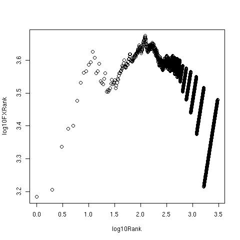
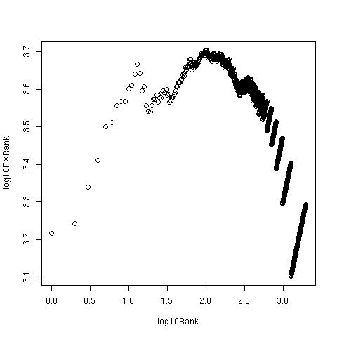
    First let me show you the Zipf plots for the text as we sequentially process it. Recall from the post on To Zipf or not to Zipf that it is a plot of the log of the product of the frequency and rank for any token vs log(rank). We expect it to be linear, indicating a negative power law dependence of the frequency on the rank.

    All processing is done using Python code, which also creates data files and calls R for plotting. When I get my hands on real data, the R program can also fit the data to Zipf's law or Mandelbrot's law, which will help with identifying the deviations from expected linear behaviour and the ranks at which we establish the 'stop' and 'rare' cut-offs. (To see more details of the figures and tables, click on them.)
    Zipf Plot of Alice, original text
      From right to left, the different segments correspond to tokens which appear only once, then those that appear twice, thrice etc. The most frequent word 'the' sits at the bottom left corner. With a large corpus, we expect the curve to be smoothed out, especially in the middle.

    Zipf Plot of Alice, text with punctuation removed

    Zipf Plot of Alice, lowercased text

    Zipf Plot of Alice, histogram of stemmed tokens

    Zipf Plot of Alice, histogram with 100 stop words removed


  8. These 100 'stop' words are just the 100 most frequent words in the text itself. As I have explained in the Zipf post, the cut off should be based on the histogram of the entire corpus.
     Again, this is for illustration purposes only.
    Zipf Plot of Alice, histogram with 20 rare words removed
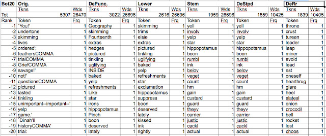
    Now, let's take a look at the 20 top and 20 bottom ranked tokens in Alice, and see how this list changes with processing.
    Top 20 Tokens
    Bottom 20 Tokens
     Summarizing,
    The above steps suffice for spell-checked and edited works, the following steps need to be implemented for user provided text.
  1.  Expand any recognizable abbr to its most likely form, so there is no remaining ambiguity. (I am not sure about this step, but presumably it involves looking up some standard dictionary.) From the remaining sequences of letters, identify the non-words and check if there are any likely words in the dictionary that could have been misspelled as the non-word. For example, consider the non-word 'mnager'. Let's say that 'manager' is likely to be misspelled as 'mnager' (dropped letter 'a') 5% of the time (where the probabilities over all result words – spellings and misspellings – of the source word 'manager' sum to 1), whereas 'manger' is likely to be misspelled as 'mnager' ('a' and 'n' transposed dyslexically) 10% of the time. These are not the probabilities to consider and thence assign 'mnager' to 'manger'. Since 'manager' is a much more frequently used word than is 'manger', 'mnager' is much more likely to be a misspelling of 'manager'. So we want to look at the probabilities that 'mnager' results as a misspelling of a source word ('manager' or 'manger'), where the sum over all source words equals 1, and then select the most likely source. Hence 'mnager' would be assigned to 'manager', unless one were to have additional information, e.g. that the text is biblical in nature.
  2. Toss out 'fzdurq' and other non-words., so that all remaining sequences of letters are words.
    These last two complicated steps can be substituted by the step of simply removing the letter sequences which are least frequent in the corpus, which are either terms from highly specialized jargon, mis-spellings or abreviations.
So you see how “To be, or not to be, that is the question:” is rendered “question”. The corpus of the text remains; ready for some numerical, but not literary, analysis.

NTA1: NumericalTextAnalysisPreliminaries

Numerical Text Analysis 1
Guide to all Text Analysis Posts

Prev: Sample Text

Definitions and Text Operations:

Text atoms: Uppercase letters (L), lowercase letters (u), punctuation marks (?), numerals (4).
Accent Marks: None in English, just consider accented letters as independent letters?
Whitespace: space, tab, newline, end-of-line, end-of-file.
Word: A sequence of text atoms; in text, preceded and succeeded by whitespace.
Text: A sequence of text atoms and whitespace. Equivalently, a sequence of words separated by whitespace. Text space is a linear space.
Corpus: A collection of texts.
Word list: a list of words, order usually does not matter. It is generated either fro a text or from another list.
Dictionary word: A word found in a dictionary or in one of a set of dictionaries.

Parse: (By default on whitespace, but a parse map can be defined for any sequence of words.) This is an operation that acts on text and generates a list of words, so parse is not in fact a text operation. It maps a point from one space into another.

Various operations can be carried out on text (or on lists, since each element of a list is text), the ones relevant for our purposes are:

Lower: Acts on any piece of text, converts all uppercase letters to the corresponding lowercase ones.
lower(upper's and(?) LOWER) = upper's and(?) lower

DePunctuate: Almost all punctuation in normal English text is juxtaposed with whitespace (WJPMs). Punctuation marks which are normally juxtaposed with whitespace can either be deleted or replaced with whitespace, in either case one will be left with just whitespace. The two exceptions are the hyphen '-' and the apostrophe “'”. '-' occours in hyphenated words like 'super-talented', which are composed of independent words. Hence the hyphen should be replaced by a whitespace. The apostrophe occours in possessives and contractions, e.g. “dog's”, “she'd” and “isn't”. In order to not create single letter words and peculiarities like “isn”, the apostrophe should be deleted. Note that stemming leaves unchanged all three of 'isn', 'isnt' and 't', and hence can't be used to make a choice. With either choice for eliminating the WJPMs, we will have one exception, either the hyphen or the apostrophe. For simplicity, let us delete the WJPMs without replacement, delete the apostrophe without replacement as well, and replace the hyphen with whitespace.
DePunctuate(“The dog's bone was super-tasty! Wasn't it?” she asked.) = The dogs bone was super tasty Wasnt it she asked

Chop[n]: Eliminates words of length n or less, with possible exceptions like 'i' and 'a' for n = 1.
Chop[2](To be or not to be, that is the question.) = not be, that the question.
I thought of this as a short cut to stop. With the choice of depunctuate above that punctuation marks (except for '-', which is replaced by whitespace) are simply deleted, there shouldn't be single letter words other than 'i' and 'a'. Having rethought stop, chop became superfluous.

Stem: Acts on a word and returns its stem. Conjugations of verbs, plurals, adjectives, adverbs and other modifiers often have the same stem. Note that the result of stem on a regular English word is not necessarily a dictionary word – it is only the sequence of letters identified as the stem. There are many stemming algorithms. I've used Porter2 from the Python implementation by Matt Chaput.


I had misunderstood the purpose of stem, and when I saw words like veget and readabl I wrote ifstem so it would only replace a word by its stem if the stem was a dictionary word.

Stop[rank]: Eliminates words whose tokens rank higher (are more frequent) than rank. See
StopWordsToBeOrNotToBeZipf Post to appear in the next day or two.

Derarify[rank from bottom]: Eliminates words whose tokens are very low-ranking by frequency. See
StopWordsToBeOrNotToBeZipf

SpellCheck: Not thought about this yet. Eliminating the least frequent tokens –DeRarifying– should take care of some mis-spellings.

ImProper: Identify and eliminate proper nouns. While any one given text may have a few names that occur with high frequency (for example in Alice in Wonderland the name Alice is the 10th ranked word), over the whole corpus most proper nouns should be relative rarities and can be eliminated by DeRarifying the text. The most common proper nouns can perhaps be listed and eliminated separately.

Histogram: Again, this is not a text operation, in fact it acts on a wordlist and returns a list of tuples or a dictionary (list of key:value pairs) whose first elements or keys are the members of the set constructed from the elements of the list and the second elements or values are the number of times they occur in the list. The space of word histograms is linear, has a natural origin and is non-negative, it is a whole-number valued “vector space”. So lets call these things “word vectors”. For any given text, then, one can construct its word vector.

The above operations don't commute with each other, hence the order in which they are carried out will affect the result.

Note for further thought: the above operations are linear operators on a linear space, and they do have eigenvalues and eigenvectors. But the operators are not all symmetric, and some of their eigenvectors lie outside text space. E.g. pure lower case text are eigenvectors of lower with eigenvalue 1. A word vector consisting of lowercase text low and equal and opposite frequencies of occurrence of text whose lowercase is low (e.g. lOw, LOW) is an eigenvector with eigenvalue 0. (See my future post on how to extend text space to make some of these operators symmetric.)

NTA0: SampleTextForAnalysis

Numerical Text Analysis 0
Guide to all Text Analysis posts

Try and guess the text I am going to use as an illustrative example. At a certain stage of text-processing, it has somewhat fewer than 2,000 word-tokens and a total length of a bit less than 27,000 words. I rank these 2,000 word tokens by order of frequency of appearance in the text. Here are some of the salient tokens and their ranks in increasing order: scan the tokens one at a time, and stop when you guess the text they are from. Give your points corresponding to the rank of the word you stopped at and report back to me via a comment.


Here is more information about the words:


The word 'head' appears only 4/5 of the times that the word 'queen' does. Assuming that 'head' appears half the time in neutral circumstances, the Queen is only yelling “Off with his head!” 2/5 of the times she makes an appearance.

The full text can be found here.

Thursday, March 22, 2012

NTA4: WordHistogramsOrHamlet{question:1}

Numerical Text Analysis 4

Guide to All text Analysis posts

Prev: Selecting Stop Tokens

WordHistogramsOrHamlet{question:1}

Consider the space of word-vectors:
  1. If there are D different word tokens in the entire collection of texts under consideration, then word-vector space is D-dimensional.
  1. It is a linear space, but it is not exactly a vector space: Though there is an origin or 0-vector (null-texts), word-vectors do not have additive inverses that I can interpret. Hence there is no subtraction defined on the space of word-vectors. Hence word-vector space is the D-dimensional positive 1/2D-ant.
2. Two texts are equivalent if they have the same word histogram, i.e. the same distribution of the frequencies of occurrence of the stemmed, non-stop word-tokens. Word-vectors are then equivalence classes of texts. 

For example, of the following 3 texts, Text A and B are equivalent to each other, but not to Text C.

Text A: This “teXt” is equivalent to the following text, Not the preceding one?

Text B: The preceding text IS equivalent to “this one”, but not to the following texts.

Text C: “This text” is not the same as the preceding one, and has no following text.

After removing punctuation, lowercasing, stemming and removing stop words, their histograms are A: {text: 2, preced: 1, follow: 1, equival: 1}, 
B: {text: 2, preced: 1, follow: 1, equival: 1} and 
C: {text: 2, preced: 1, follow: 1, equival: 0}.

  1. Two word-vectors can be added to each other, and they can be scaled by positive integers. If we define the '+' of two texts to be the text formed by writing one text followed by the other, then
    vec(Text D) + vec(Text E) = vec(Text D '+' Text E)
  2. You can effectively divide a word-vector V by a positive integer q (and hence scale by positive rationals) by leaving V alone and scaling all the rest by q.

If we normalize all word-vectors to unit magnitude (i.e. as vectors, so the sum of the squares of the frequencies is 1), then the resulting space is the positive 1/2D-1-sphere and texts are now points on this hemisphere.

However, we could also normalize the word-histograms, so the sum of the frequencies themselves – not the sum of their squares – is 1. In this case the resulting space is the D-1 simplex, which is tangent to the sphere at (1, 1, 1, …). Note that the space of probabilities for the occurrence of D mutually exclusive events is a D-simplex, and that word-histograms have a natural probabilistic interpretation but not an obvious interpretation as vectors. So in most cases we will prefer to live on the simplex and not the sphere.

What does text-space look like? I want you to imagine yourself at the origin, at the point corresponding to the null-text. Small texts with few words are close by and large texts are further away. All 'normal' texts are in the positive 2-D-ant (π/2 radians in 2D and π steradians in 3D etc.). Similar texts are along the same line of sight and very dissimilar texts will be at large angles to each other, up to a maximum of 90 degrees. Whether we've normalized the texts as vectors (on the unit sphere) or as histograms (on the unit simplex), the angles between them as viewed from the origin are the same. 
 
The word histogram for the first line of Hamlet's soliloquy at the beginning of Act 3 Scene 1 of the eponymous play is {question: 1}.

Still fairly simple undergrad or even high school CS skills (based on the really smart interns at LinkedIn during the summer of 2011) and perhaps a graduate numerical text analysis course.

Next: An aside Word Play
or see the word histogram for the corpus